Text Segmentation: A Closer Look at Clustering and Beyond
This is the third installment in a series about text segmentation. The first part covered text segmentation metrics, and the second focused on unsupervised text segmentation methods.
When I began writing this article, I had a strong belief that employing clustering was an excellent approach to segment text into distinct topics. Regrettably, it turned out that I was mistaken. Perhaps I overlooked something crucial, which is why this approach yielded no meaningful results.
On the other hand I tried multiple dimention reduction techniques and got a lot of beautiful graphics that show my failure.
I had two goals to investigate:
- Grouping sentences about a topic in a podcast episode into one cluster.
- Distinguishing between sentences within a topic and sentences that start a new discussion, and creating two clusters accordingly.
However, when I visualized the embeddings and examined the plots, it was evident that there were no clear boundaries between topics. This indicated that using clustering for text segmentation wouldn’t be straightforward. It appears that more research is needed, and I hope to dedicate more time to it later.
By the way, this little research provided an opportunity to experiment with new visualization techniques and dimension reduction methods. So instead of focusing solely on text segmentation methods, this article has transformed into one about embeddings visualization and dimension reduction techniques.
In this article, I’ll examine three dimension reduction techniques: t-SNE, PCA, and UMAP. For each technique, I’ll create various scatter plots based on the objectives I mentioned earlier and specific options related to each method.
Disclaimer: I won’t go into detailed algorithmic explanations in this article, but I’ll strive to provide simplified explanations of the core concepts behind these methods.
Setup
As I’ve previously discussed, I’m using transcripts from the DevZen podcast. Specifically, I’ve selected the 412th episode randomly. In this article, I’ll focus on visualizing and attempting to cluster sentences from this particular episode.
To start, I’ll import all the essential libraries and generate embeddings for the upcoming analysis.
import typing as t
from dataclasses import dataclass
import re
import warnings
warnings.filterwarnings("ignore")

from joblib import Memory

import pandas as pd
import numpy as np

import matplotlib.pyplot as plt
import plotly.express as px
import plotly.graph_objs as go
from plotly.subplots import make_subplots

from tqdm.notebook import tqdm

from stop_words import get_stop_words
from sentence_transformers import SentenceTransformer
memory = Memory('../.cache')
csv_path = '../data/400-415-episodes-ground-truth.csv'
df = pd.read_csv(csv_path)
df = df[df['episode'] == 412]
df.head()
| size | episode | start | end | ru_sentence | sentence_length | topic_num | ground_truth | en_sentence | |
|---|---|---|---|---|---|---|---|---|---|
| 13289 | medium | 412 | 0.00 | 11.40 | Всем привет! | 12 | 1 | 1 | Hi all! |
| 13290 | medium | 412 | 0.00 | 11.40 | Вы слушаете подкаст DevZen выпуск номер 412, з... | 76 | 1 | 1 | You listen to the Devzen podcast issue number ... |
| 13291 | medium | 412 | 11.40 | 19.08 | Записываемся как всегда полным составом, кроме... | 65 | 1 | 1 | We sign up as always with a full composition, ... |
| 13292 | medium | 412 | 11.40 | 25.20 | Подкаст теперь есть на Spotify, если вы пропус... | 68 | 1 | 1 | There is now a podcast on Spotify if you misse... |
| 13293 | medium | 412 | 19.08 | 25.20 | А со мной этот подкаст ведет Валера. | 36 | 1 | 1 | And with me this podokast is leading Valera. |
Just a friendly reminder of the column meanings:
size: Size of the model used to transcribe an episode.episode: Episode number.startandend: Start and end timings for each sentence respectively. Some sentences may have overlapping timings due to a limitation during transcription.ru_sentence: Original sentence in Russian.en_sentence: Machine-translated original sentence in English.sentence_length: Length of the original sentence.topic_num: Topic number from the episode’s show notes.ground_truth: Manually set topic number.
Prepare embeddings
Similar to the segmentation article, I’ll utilize the SentenceTransformers library to construct embeddings and Plotly for visualization.
For embeddings, I’ll utilize two multilanguage models: paraphrase-multilingual-MiniLM-L12-v2 and labse. I’ll experiment with various parameters for each dimension reduction algorithm.
@dataclass
class Models:
    paraphrase = 'sentence-transformers/paraphrase-multilingual-MiniLM-L12-v2'
    labse = 'sentence-transformers/labse'
@memory.cache
def get_embeddings(sentences: list[str], model_name: str) -> list[float]:
    model = SentenceTransformer(model_name)
    return model.encode(sentences)
ru_paraphrase_embeddings = get_embeddings(df['ru_sentence'].values, Models.paraphrase)
en_paraphrase_embeddings = get_embeddings(df['en_sentence'].values, Models.paraphrase)

ru_labse_embeddings = get_embeddings(df['ru_sentence'].values, Models.labse)
en_labse_embeddings = get_embeddings(df['en_sentence'].values, Models.labse)
print(f'{ru_paraphrase_embeddings.shape=}')
print(f'{en_paraphrase_embeddings.shape=}')

print(f'{ru_labse_embeddings.shape=}')
print(f'{en_labse_embeddings.shape=}')
ru_paraphrase_embeddings.shape=(1330, 384)
en_paraphrase_embeddings.shape=(1330, 384)
ru_labse_embeddings.shape=(1330, 768)
en_labse_embeddings.shape=(1330, 768)
embeddings = {
    'russian': {
        'paraphrase': ru_paraphrase_embeddings,
        'labse': ru_labse_embeddings,
    },
    'english': {
        'paraphrase': en_paraphrase_embeddings,
        'labse': en_labse_embeddings,
    }
}
The initial model, paraphrase-multilingual-MiniLM-L12-v2, produces embeddings with 384 dimensions, while the second model, labse, yields 768-dimensional embeddings.
Prepare dataset
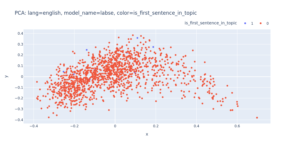
To accomplish the second objective, I’ll use a bit of pandas ✨magic✨ to label each sentence in the dataset as either an “inner topic sentence” or a “first topic sentence.”
df['ground_truth_next'] = df['ground_truth'].shift(1).fillna(df['ground_truth'].max()).astype(int)
def is_first_sentence_in_topic(s: pd.Series) -> int:
    return 0 if s['ground_truth'] == s['ground_truth_next'] else 1

df['is_first_sentence_in_topic'] = df.apply(is_first_sentence_in_topic, axis='columns')
df[df['is_first_sentence_in_topic'] == 1][['ru_sentence', 'en_sentence', 'ground_truth', 'is_first_sentence_in_topic']]
| ru_sentence | en_sentence | ground_truth | is_first_sentence_in_topic | |
|---|---|---|---|---|
| 13289 | Всем привет! | Hi all! | 1 | 1 |
| 13620 | Я думаю, Алекс просто скромничает, потому что ... | I think Alex is just modest, because he came t... | 2 | 1 |
| 13630 | Спасибо, у меня тоже есть эраты, мы раньше гов... | Thank you, I also have erata, we used to talk ... | 3 | 1 |
| 13636 | Кто еще офигевает? | Who else is coming out? | 4 | 1 |
| 13806 | Это тема, которую я видел на хабре несколько н... | This is the topic that I saw on Habria a few w... | 5 | 1 |
| 14057 | Следующая тема про Executives. | The next topic about executives. | 6 | 1 |
| 14217 | Когда очередной как-то, есть такой productivit... | When another one, there is such a Productivity... | 7 | 1 |
| 14359 | Что еще можно показать? | What else can be shown? | 8 | 1 |
| 14444 | Что еще можно развернуть вполне, эта тема в за... | What else can be expanded, this topic is not i... | 9 | 1 |
| 14492 | А что еще у меня в коротких темах, это доклады... | And what else do I have in short topics are re... | 10 | 1 |
| 14544 | Ну и ладно, пойдем тогда по темам наших слушат... | Well, okay, then let's follow the topics of ou... | 11 | 1 |
color_columns = ['ground_truth', 'is_first_sentence_in_topic']
From here I can start my research.
PCA
Principal component analysis (PCA) is a popular technique for analyzing large datasets containing a high number of dimensions/features per observation, increasing the interpretability of data while preserving the maximum amount of information, and enabling the visualization of multidimensional data. Wikipedia
This algorithm identifies the directions in the data where it varies the most. It then projects the data onto these directions (principal components), which are orthogonal and ordered by the amount of variance they explain. This transformation allows for a more compact representation of the original data while retaining its essential features.
Here is a video from the StatQuest channel below. The creator provides a more comprehensive explanation of PCA along with examples.
Disclaimer #2: I have no information about the creator of the StatQuest channel; I’m just providing a link to the video.
from sklearn.decomposition import PCA
def pca_scatter(embeddings: list[float], title: str, color_column: str) -> None:
pca = PCA(n_components=2, random_state=42)
pca_embeddings = pca.fit_transform(embeddings)
pca_df = pd.DataFrame(pca_embeddings, columns=('x', 'y'))
pca_df = df.join(pca_df.set_index(df.index))
pca_df[color_column] = pca_df[color_column].astype(str)
fig = px.scatter(
title=f'PCA: {title}',
data_frame=pca_df,
x='x',
y='y',
color=color_column,
hover_data=['ru_sentence', 'en_sentence'],
width=1000
)
fig.update_layout(legend=dict(
orientation='h',
yanchor="bottom",
y=1.02,
xanchor="right",
x=1
))
return fig
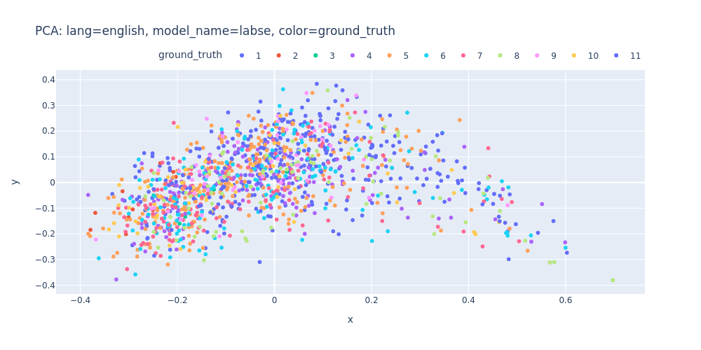
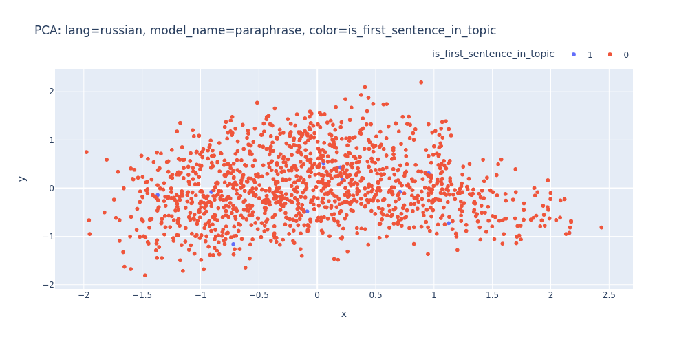
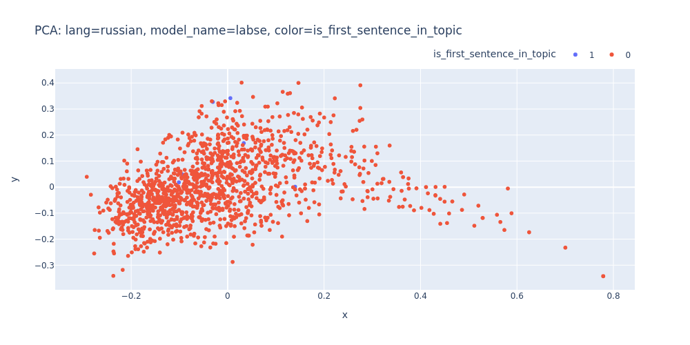
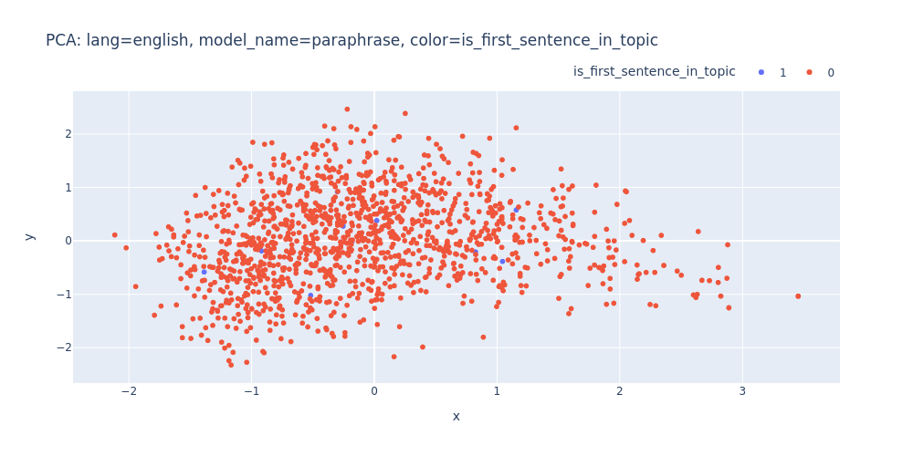
for color_column in color_columns:
for lang, embedding_pairs in embeddings.items():
for model_name, embedding in embedding_pairs.items():
pca_scatter(
embeddings=embedding,
title=f'lang={lang}, model_name={model_name}, color={color_column}',
color_column=color_column).show(renderer='png')
lang=russian-model_name=paraphrase-color=ground_truth.html
lang=russian-model_name=labse-color=ground_truth.html
lang=english-model_name=paraphrase-color=ground_truth.html
lang=english-model_name=labse-color=ground_truth.html
lang=russian-model_name=paraphrase-color=is_first_sentence_in_topic.html
lang=russian-model_name=labse-color=is_first_sentence_in_topic.html
lang=english-model_name=paraphrase-color=is_first_sentence_in_topic.html
lang=english-model_name=labse-color=is_first_sentence_in_topic.html
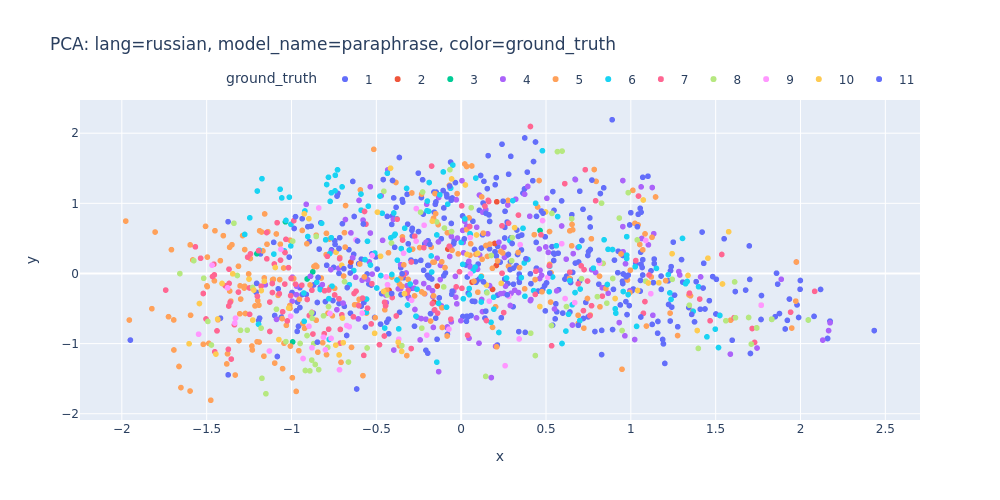
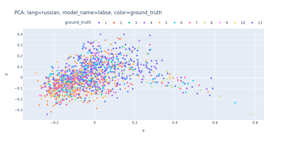
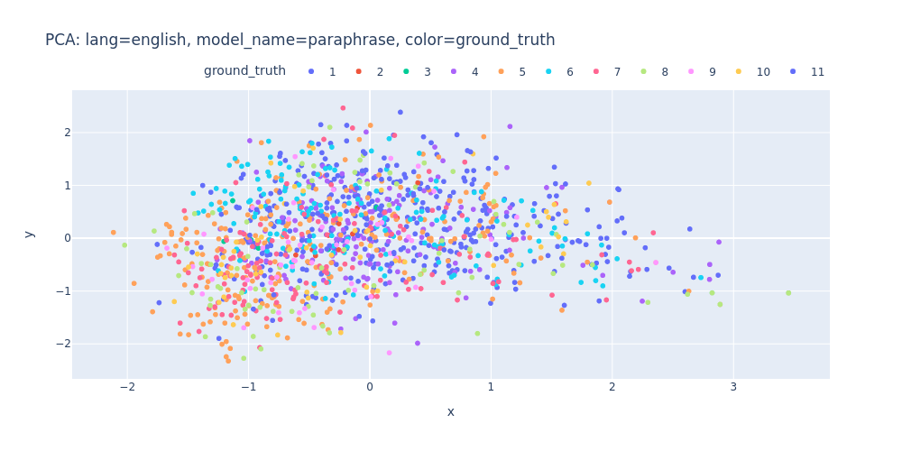
As observed, PCA does not effectively assist in segregating topics into distinct clusters — neither into 11 clusters for each topic nor into 2 clusters for first/inner sentences.
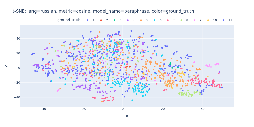
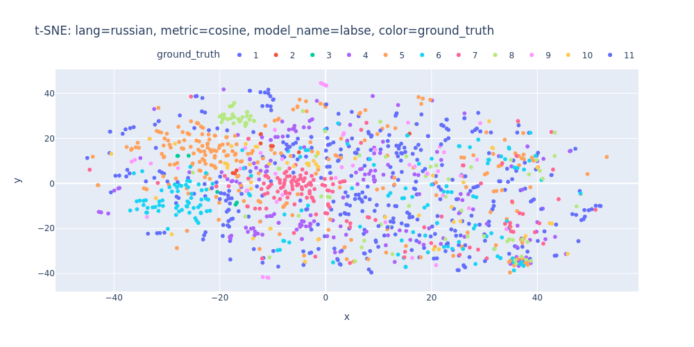
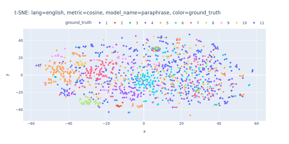
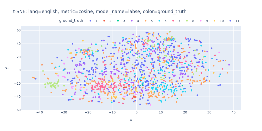
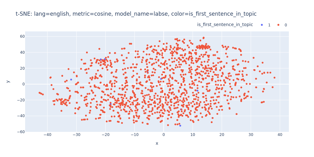
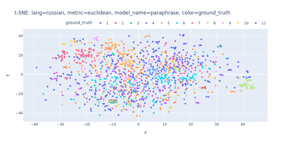
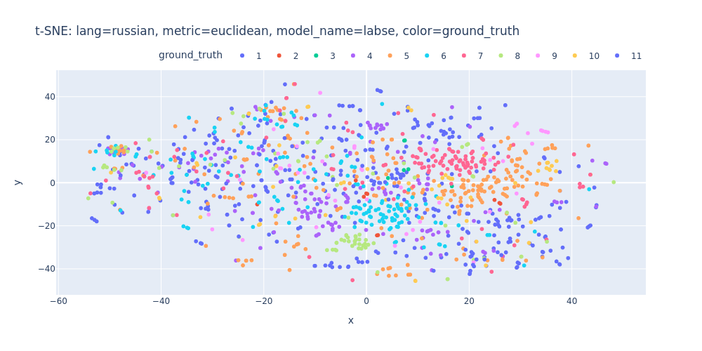
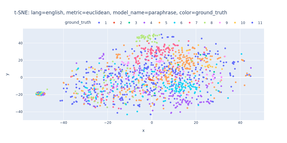
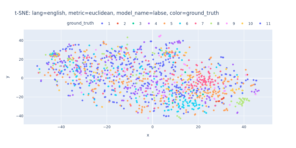
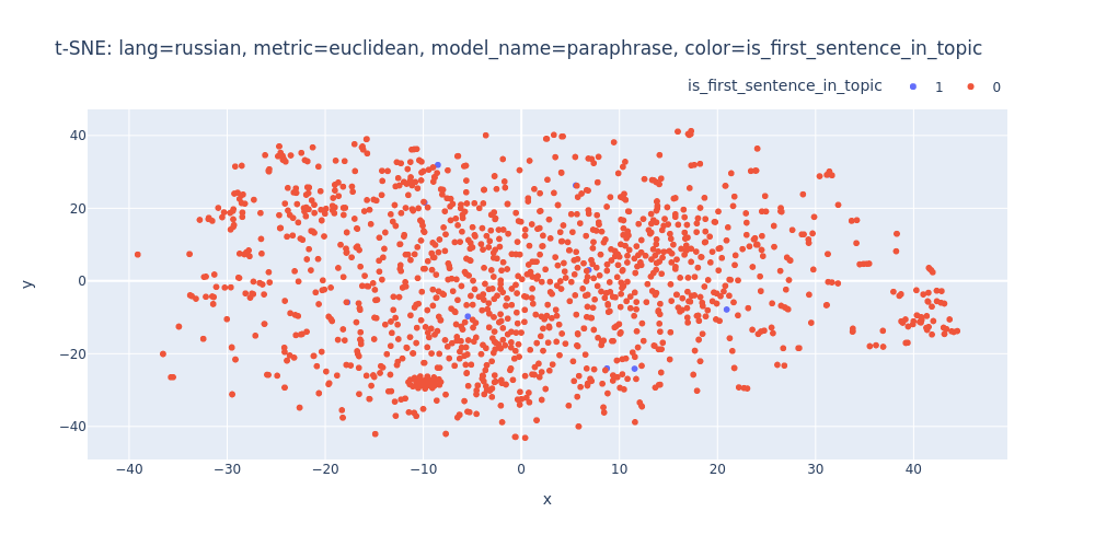
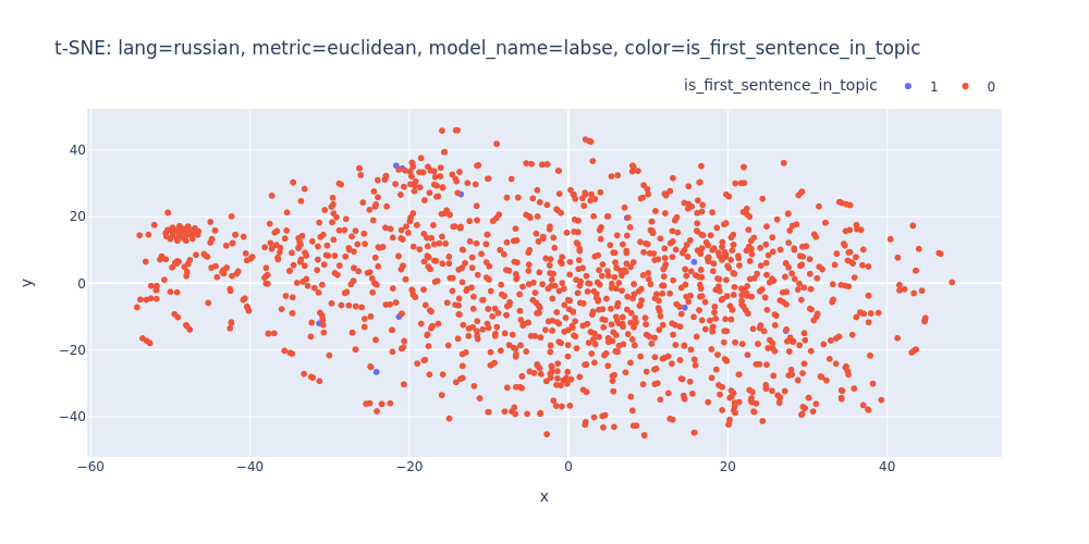
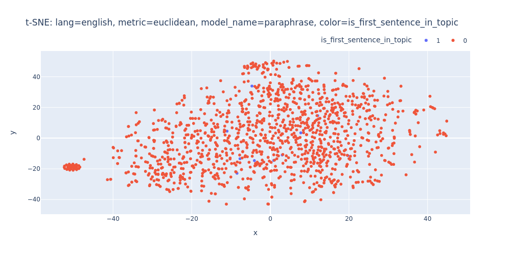
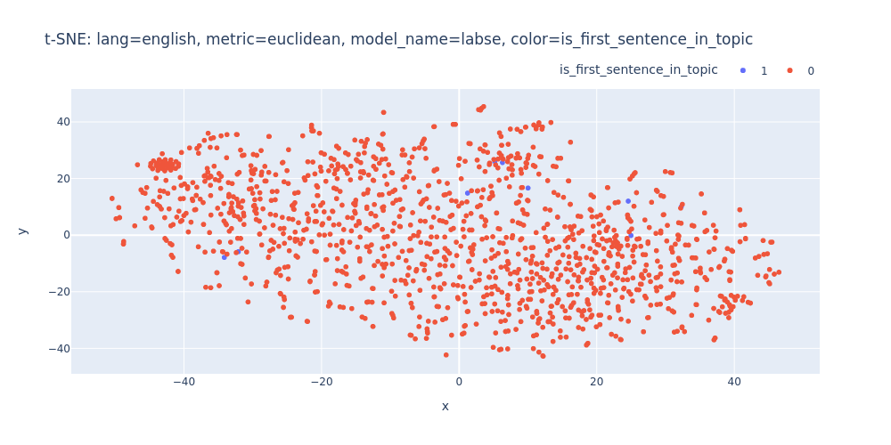
t-SNE
t-distributed stochastic neighbor embedding (t-SNE) is a statistical method for visualizing high-dimensional data by giving each datapoint a location in a two or three-dimensional map. Wikipedia
I may not be able to explain the entire algorithm in detail, but in essence, it helps transform data into a representation where similar instances are nearby and dissimilar ones are far apart. This is achieved by optimizing the match between pairwise similarities in the original high-dimensional space and the lower-dimensional representation.
To see the algorithm in action with a simple example, you can watch the video below from StatQuest:
from sklearn.manifold import TSNE
from scipy.spatial.distance import cosine


@memory.cache
def tsne_transform(embeddings: list[list[float]], metric: t.Union[str, t.Callable], early_exaggeration: int):
    tsne = TSNE(n_components=2, metric=metric, random_state=42, early_exaggeration=early_exaggeration, n_jobs=-1)
    tsne_embeddings = tsne.fit_transform(embeddings)
    return tsne_embeddings

def tsne_scatter(embeddings: list[list[float]], metric: t.Union[str, t.Callable], title: str, color_column: str) -> None:
    tsne_embeddings = tsne_transform(embeddings=embeddings, metric=metric, early_exaggeration=20)

    tsne_df = pd.DataFrame(tsne_embeddings, columns=('x', 'y'))
    tsne_df = df.join(tsne_df.set_index(df.index))
    tsne_df[color_column] = tsne_df[color_column].astype(str)

    fig = px.scatter(
        title=f't-SNE: {title}',
        data_frame=tsne_df,
        x='x',
        y='y',
        color=color_column,
        hover_data=['ru_sentence', 'en_sentence'],
        width=1000)

    fig.update_layout(legend=dict(
        orientation='h',
        yanchor="bottom",
        y=1.02,
        xanchor="right",
        x=1
    ))

    return fig
In contrast to PCA, t-SNE supports various similarity metrics. In my case, I tested two of them: scipy.spatial.distance.cosine and the default euclidean.
metrics = {
    'cosine': cosine,
    'euclidean': 'euclidean',
}
for metric_name, metric in metrics.items():
    for color_column in color_columns:
        for lang, embedding_pairs in embeddings.items():
            for model_name, embedding in embedding_pairs.items():
                tsne_scatter(
                    embeddings=embedding,
                    metric=metric_name,
                    title=f'lang={lang}, metric={metric_name}, model_name={model_name}, color={color_column}',
                    color_column=color_column).show(renderer='png')
lang=russian-metric=cosine-model_name=paraphrase-color=ground_truth.html
lang=russian-metric=cosine-model_name=labse-color=ground_truth.html
lang=english-metric=cosine-model_name=paraphrase-color=ground_truth.html
lang=english-metric=cosine-model_name=labse-color=ground_truth.html
lang=russian-metric=cosine-model_name=paraphrase-color=is_first_sentence_in_topic.html
lang=russian-metric=cosine-model_name=labse-color=is_first_sentence_in_topic.html
lang=english-metric=cosine-model_name=paraphrase-color=is_first_sentence_in_topic.html
lang=english-metric=cosine-model_name=labse-color=is_first_sentence_in_topic.html
lang=russian-metric=euclidean-model_name=paraphrase-color=ground_truth.html
lang=russian-metric=euclidean-model_name=labse-color=ground_truth.html
lang=english-metric=euclidean-model_name=paraphrase-color=ground_truth.html
lang=english-metric=euclidean-model_name=labse-color=ground_truth.html
lang=russian-metric=euclidean-model_name=paraphrase-color=is_first_sentence_in_topic.html
lang=russian-metric=euclidean-model_name=labse-color=is_first_sentence_in_topic.html
lang=english-metric=euclidean-model_name=paraphrase-color=is_first_sentence_in_topic.html
lang=english-metric=euclidean-model_name=labse-color=is_first_sentence_in_topic.html
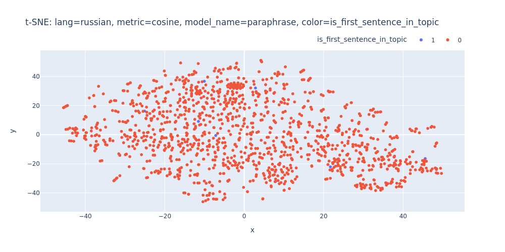
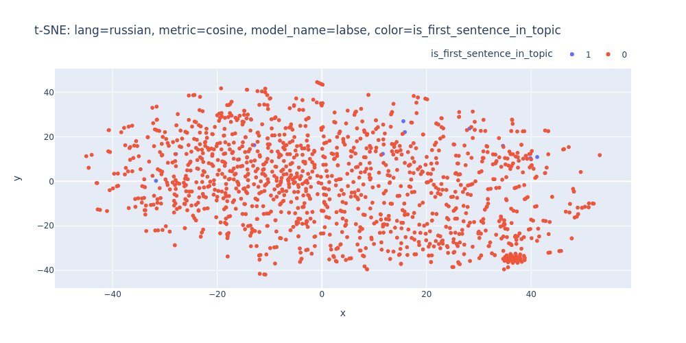
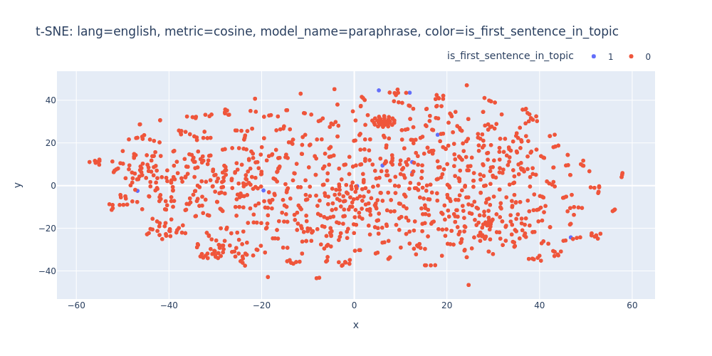
Unfortunately, t-SNE also didn’t assist me in visualizing distinct differences between topics or identifying first/inner sentences within a topic.
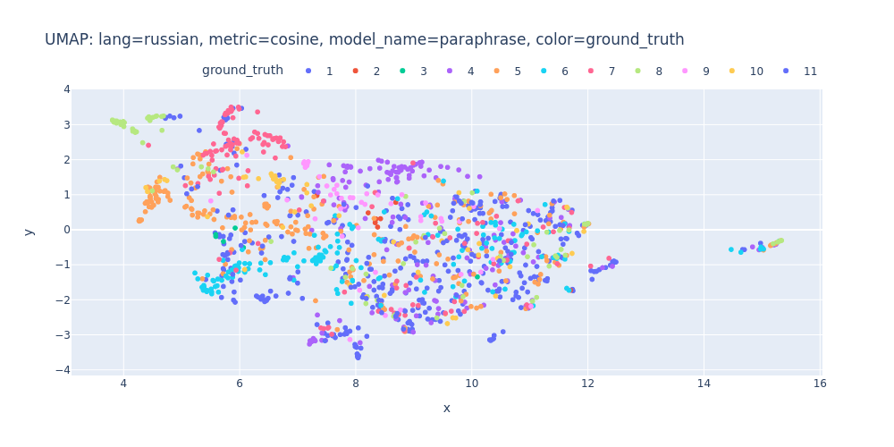
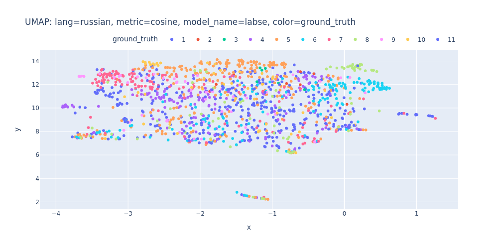
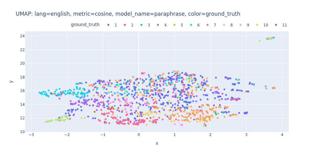
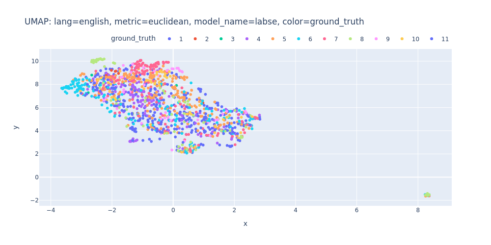
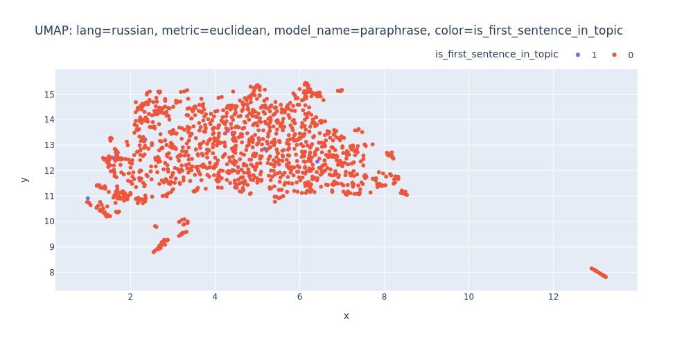
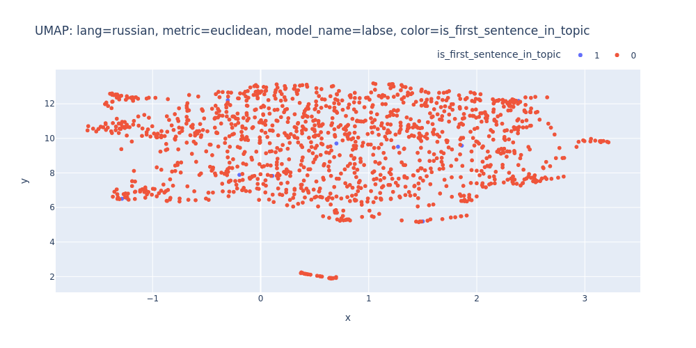
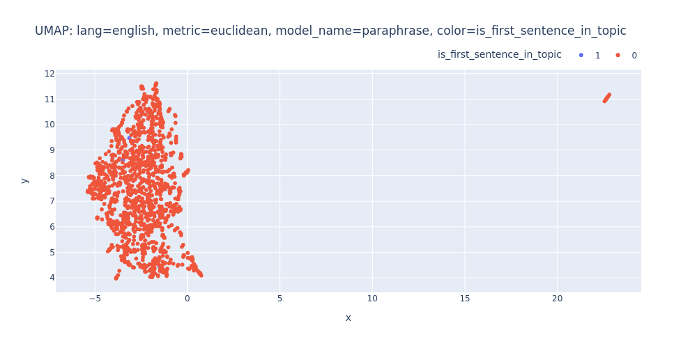
UMAP
UMAP (Uniform Manifold Approximation and Projection) is a novel manifold learning technique for dimension reduction. UMAP is constructed from a theoretical framework based in Riemannian geometry and algebraic topology. The result is a practical scalable algorithm that applies to real world data. The UMAP algorithm is competitive with t-SNE for visualization quality, and arguably preserves more of the global structure with superior run time performance. Furthermore, UMAP has no computational restrictions on embedding dimension, making it viable as a general purpose dimension reduction technique for machine learning. arXiv
UMAP is a modern dimension reduction technique, and you can find a helpful video about the algorithm on StatQuest’s YouTube channel:
import umap


@memory.cache
def umap_transofrm(embeddings: list[list[float]], metric: t.Union[str, t.Callable]):
    umap_reducer = umap.UMAP(n_neighbors=15, min_dist=0.1, n_components=2, metric=metric)
    umap_embeddings = umap_reducer.fit_transform(embeddings)
    return umap_embeddings


def umap_scatter(embeddings: list[float], metric: t.Union[str, t.Callable], color_column: str, title: str):
    umap_embeddings = umap_transofrm(embeddings, metric)

    umap_df = pd.DataFrame(umap_embeddings, columns=('x', 'y'))
    umap_df = df.join(umap_df.set_index(df.index))
    umap_df[color_column] = umap_df[color_column].astype(str)

    fig = px.scatter(
        title=f'UMAP: {title}',
        data_frame=umap_df,
        x='x',
        y='y',
        color=color_column,
        hover_data=['ru_sentence', 'en_sentence'],
        width=1000
    )

    fig.update_layout(legend=dict(
        orientation='h',
        yanchor="bottom",
        y=1.02,
        xanchor="right",
        x=1
    ))

    return fig
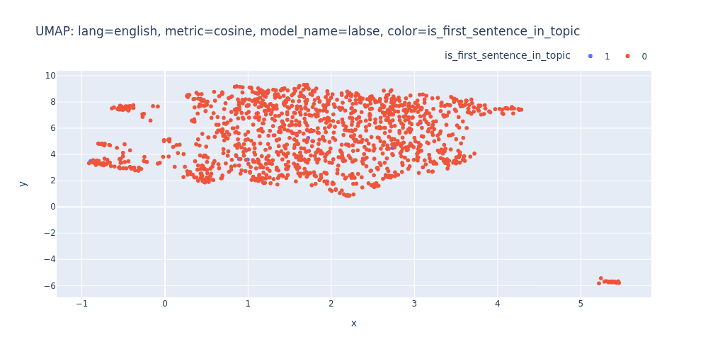
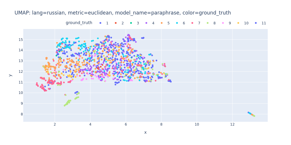
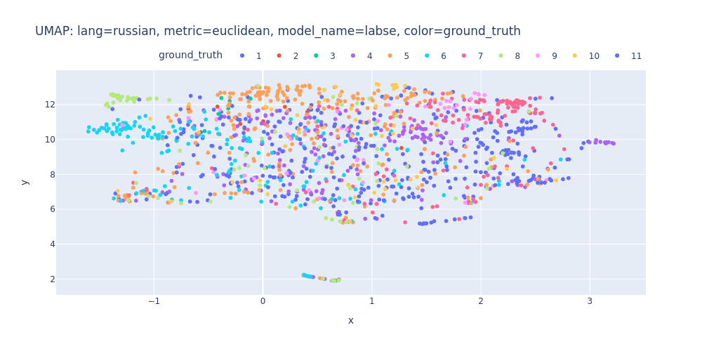
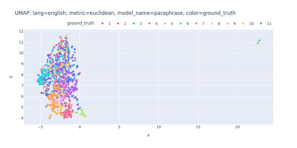
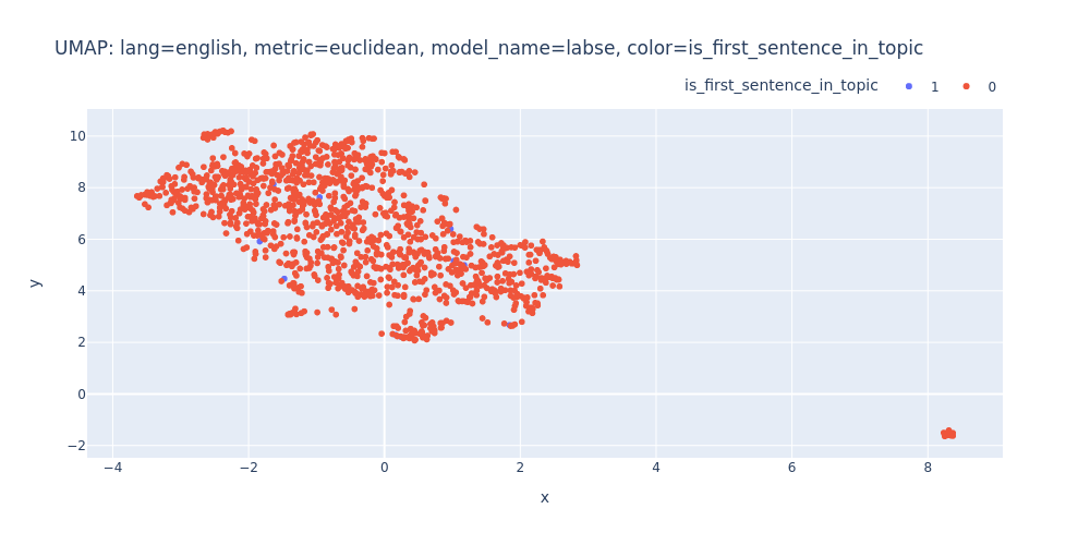
Just like t-SNE, UMAP offers various metrics for similarity computation. In my exploration, I’ll be utilizing both scipy.spatial.distance.cosine and the default euclidean.
for metric_name, metric in metrics.items():
    for color_column in color_columns:
        for lang, embedding_pairs in embeddings.items():
            for model_name, embedding in embedding_pairs.items():
                umap_scatter(
                    embeddings=embedding,
                    metric=metric_name,
                    title=f'lang={lang}, metric={metric_name}, model_name={model_name}, color={color_column}',
                    color_column=color_column).show(renderer='png')
umap-lang=russian-metric=cosine-model_name=paraphrase-color=ground_truth.html
umap-lang=russian-metric=cosine-model_name=labse-color=ground_truth.html
umap-lang=english-metric=cosine-model_name=paraphrase-color=ground_truth.html
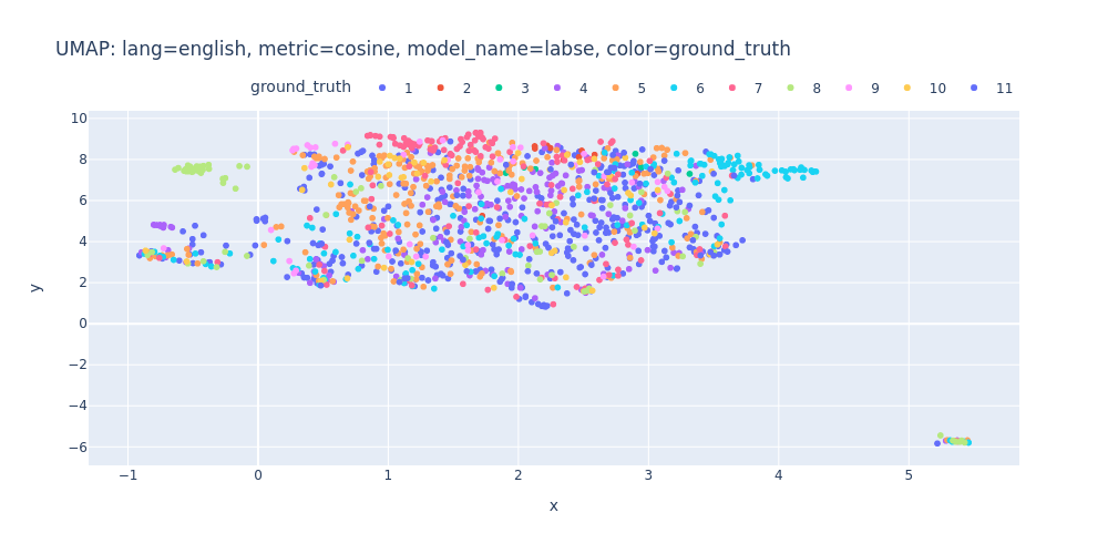
umap-lang=english-metric=cosine-model_name=labse-color=ground_truth.html
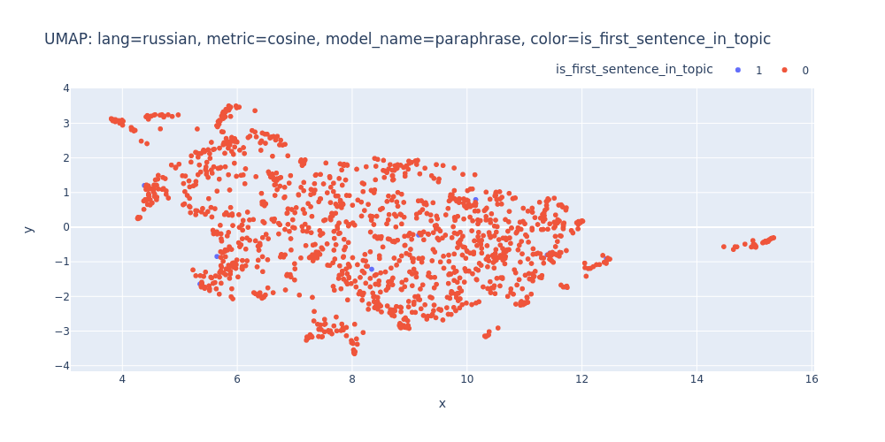
umap-lang=russian-metric=cosine-model_name=paraphrase-color=is_first_sentence_in_topic.html
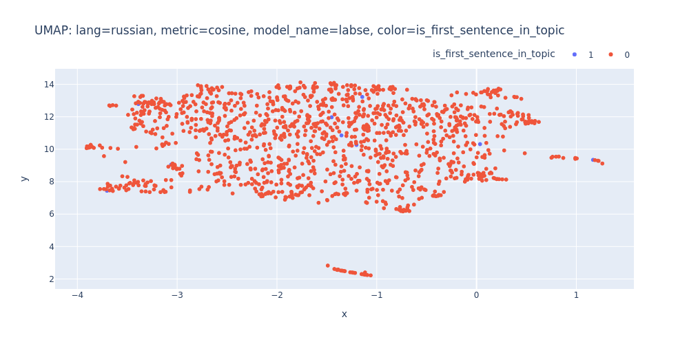
umap-lang=russian-metric=cosine-model_name=labse-color=is_first_sentence_in_topic.html
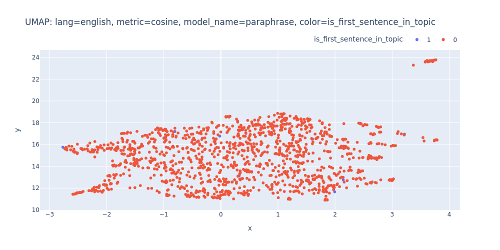
umap-lang=english-metric=cosine-model_name=paraphrase-color=is_first_sentence_in_topic.html
umap-lang=english-metric=cosine-model_name=labse-color=is_first_sentence_in_topic.html
umap-lang=russian-metric=euclidean-model_name=paraphrase-color=ground_truth.html
umap-lang=russian-metric=euclidean-model_name=labse-color=ground_truth.html
umap-lang=english-metric=euclidean-model_name=paraphrase-color=ground_truth.html
umap-lang=english-metric=euclidean-model_name=labse-color=ground_truth.html
umap-lang=russian-metric=euclidean-model_name=paraphrase-color=is_first_sentence_in_topic.html
umap-lang=russian-metric=euclidean-model_name=labse-color=is_first_sentence_in_topic.html
umap-lang=english-metric=euclidean-model_name=paraphrase-color=is_first_sentence_in_topic.html
umap-lang=english-metric=euclidean-model_name=labse-color=is_first_sentence_in_topic.html
So, there are no strong indications that we can segment the transcript into topics using just embeddings and clustering.
Conclusion
When I initially considered the concept of clustering podcast transcripts, I had high hopes for its success. Unfortunately, not all concepts lead to visible results.
On the flip side, I gained valuable experience with Plotly and various dimension reduction algorithms.
PS
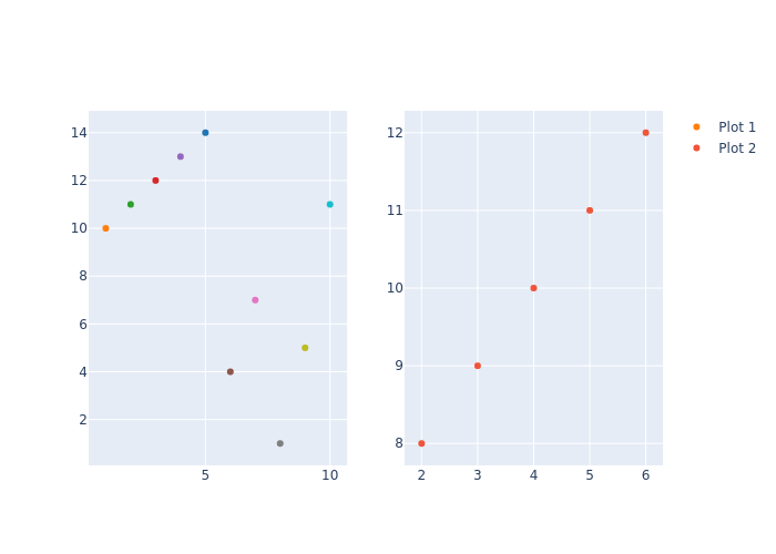
You might wonder why I created each scatter plot individually instead of using subplots. The reason is that each subplot cannot have its own individual legend. However, the interactive legend was the main factor affecting my choice of Plotly over seaborn or matplotlib:
import plotly.graph_objs as go
from plotly.subplots import make_subplots


# Create data for the scatter plots
x1 = [1, 2, 3, 4, 5, 6, 7, 8, 9, 10]
y1 = [10, 11, 12, 13, 14, 4, 7, 1, 5, 11]
z1 = [1, 2, 3, 4, 0, 5, 6, 7, 8, 9]

custom_colors = px.colors.qualitative.D3
color_scale = [custom_colors[val] for val in z1]

x2 = [2, 3, 4, 5, 6]
y2 = [8, 9, 10, 11, 12]

# Create scatter plot traces
trace1 = go.Scatter(
    x=x1,
    y=y1,
    name='Plot 1',
    mode='markers',
    marker=dict(
        color=color_scale,  # Color scale based on the Z axis
        colorscale='Viridis',  # Choose the desired colorscale (e.g., 'Viridis', 'Blues', 'reds', etc.)
    ))
trace2 = go.Scatter(x=x2, y=y2, mode='markers', name='Plot 2')

# Create a subplot
fig = make_subplots(rows=1, cols=2)

# Add the traces to the subplot
fig.add_trace(trace1, row=1, col=1)
fig.add_trace(trace2, row=1, col=2)

# Display the plot
fig.show()